Design a single trace or a differential pair and calculate its impedance.
User guide
From trace geometry to impedance and transmission.
User guide
Choose a line and prepare a project
For a pair, Z0,1 and Z0,2 describe each trace in isolation, without its neighbor's coupling. These are not Zdiff/2, which corresponds to odd-mode impedance only for symmetric pairs. Isolated values use the analytical formula or independent 2D extraction, as labeled below the readout. Numerical target dimension search and its sweep are available in both Simple and Advanced modes.
The enlarged result reads Z0 = for an isolated trace or Zdiff = for a pair, with its method below. When the geometry requires 2D solving, click the small ▶ button beside Z: only that configuration is solved at the mesh selected in the 2D panel, without tolerance studies or extra refinement. Its result and field map then appear. Geometry edits invalidate the value; calculate again. The full 2D panel can solve A, B or both with refinement and tolerances.
Use one configuration to design a line, or select Compare A and B to keep two variants side by side on desktop. Each configuration has its own line mode, geometry and target. Single-ended starts at 50 Ω; a differential pair starts at 100 Ω.
Use the top bar to change language and theme. The left menu follows the page sections. Free calculations run in your browser. Reopen a JSON project or use local save to resume work. Undo and Redo retain up to 100 project changes.
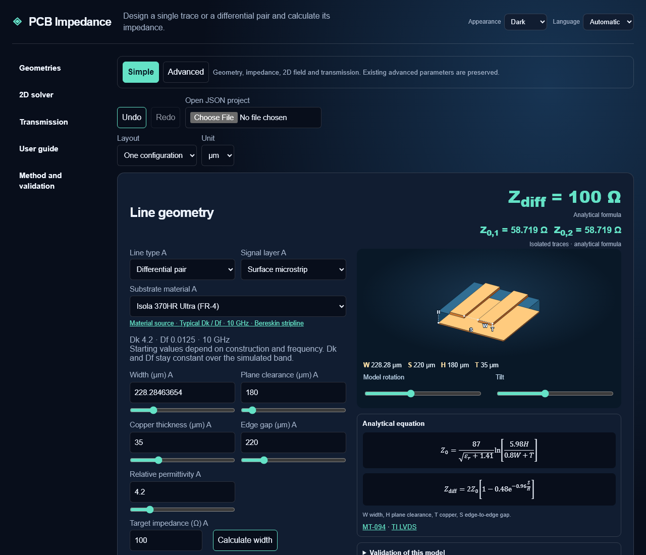
Understand dimensions and materials
W is the bottom copper width, H the clearance from the bottom of the trace to the lower reference plane, T copper thickness and S the gap between the bottom trace edges. Symmetric stripline plane separation is 2H + T. Asymmetric stripline also needs the upper plane clearance. Coplanar lines add G, the clearance to the side grounds.
Choose µm, mm or mil for cross-section dimensions. Changing units preserves the physical values; project files use mm. The impedance formulas contain length ratios, so all their dimensions must use the same unit.
Each dimension has a slider for quick exploration and a number field for precise entry. Both stay synchronized; arrow keys adjust focused sliders. Practical ranges do not guarantee applicability: the solver validates the complete cross-section.
Choose a laminate preset or enter εr. The manufacturer Dk values are starting points. Use the value for your construction and frequency. Df, entered under Transmission or imported by layer, is the dielectric loss tangent.
MEGTRON5 uses a historical manufacturer reference at 1 GHz. MEGTRON6 distinguishes glass types and measurement frequencies. EM-528, EM-528K and EM-890K distinguish RC50% and RC70%, where RC means resin content. Source and conditions are shown. Selecting a material also fills Df where available; override it under Transmission. Dk and Df stay constant across the band, without dispersion interpolation.
Set trapezoidal copper and the dielectric stackup
Open Fabrication and stackup. Top width W₂ = W − 2 × inset per side. Enter the top width directly or adjust the inset. For example, W = 300 µm and a 20 µm inset give W₂ = 260 µm. Top width must be positive and no greater than bottom width. Zero inset gives a rectangle.
The solver treats each trapezoid sidewall as a straight line, with the grid fine enough that the stair-step stays inside one cell. Drag the dimensioned 3D view with a mouse or touch; keyboard-accessible rotation and tilt sliders are also available.
Advanced pairs can set the second trace width, copper and inset independently. Broadside places traces on two levels: S is their vertical gap, H the lower-plane clearance and H₂ the clearance from the upper trace to the upper plane. Lateral offset misaligns the traces. Maps, 3D views and reports use this cross-section.
Inter-trace mask height can be specified independently above the substrate. Upper dielectric shares cover the region above the first trace and total 100%. Layer Dk and Df replace the corresponding global values.
For surface lines, enter mask thickness above copper and mask permittivity. That thickness coats the top, both sidewalls and the substrate. An optional substrate height changes only the film on the board. Lower dielectric layers run from the reference plane toward the trace and their shares must total 100%. H is their combined thickness. Fabrication models use the 2D solver.
The manufacturer CSV columns are source,copper_um,min_width_um,min_gap_um,layer,thickness_um,dk,df. Download the example in the workbench. Each row describes a dielectric; repeat copper thickness and manufacturing limits on every row. Import applies to A and B and keeps provenance. Inverse search respects the applicable minimum dimension.
Find a dimension for an impedance target
Calculate width beside the geometry inverts the analytical equation while keeping other parameters fixed. The active equation is shown below the 3D view when available.
Under Find a dimension with the 2D solver, choose the configuration and dimension. Width, copper thickness and dielectric height are available for single traces. A pair adds edge gap; buried and coplanar geometries have their specific dimensions.
Enter a target and two manufacturing bounds in µm. The solver evaluates both endpoints and uses bisection. Review the resulting dimension, impedance and signed residual before applying it. Plot sweep evaluates 13 points and marks the target and manufacturer minimum.
Diagnostics distinguish an unbracketed target, a manufacturing-limit conflict, an out-of-domain geometry and numerical nonconvergence. Endpoint results help you choose a new interval. Changing substrate height keeps imported layer proportions fixed.
Choose precision, monitor progress and cancel
Choose A, B or both, then Quick (h/8), Standard (h/16) or Fine (h/20). This sets maximum cell spacing relative to H. Finer meshes take more time and memory.
The refinement option also solves with four more cells per H: h/12, h/20 or h/24 depending on the selected precision. The impedance shown is then the first-order Richardson extrapolation of the two meshes. The nominal mesh value and the boundary shift stay visible. This is not a physical error bound.
During a run, the interface shows progress, phase and elapsed time. The estimated duration is approximate and depends on your device and geometry. Cancel calculation terminates the worker. You can then change inputs and start again.
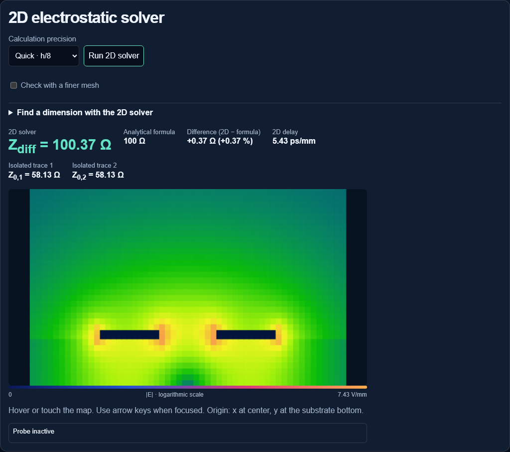
Read results and probe the field
The 2D result includes impedance, delay and comparison with an analytical equation where available. The percentage difference uses the analytical value as denominator.
Hover or touch the map to read x, y, V and |E|. Focus the map and use arrow keys for keyboard probing. x = 0 is at the cross-section center and y = 0 is at the substrate bottom. Potential is interpolated between mesh nodes; the reported field comes from the selected cell.
A single trace is driven at 1 V and a differential pair at +0.5 V and −0.5 V. Each map has its own logarithmic color scale. Peaks near corners depend on the mesh and should not be used to predict breakdown.
Validation of this model describes available comparisons. Polar, Cohn and CPW examples cover individual cases. Geometries awaiting an independent reference are identified. Read Method for equations and assumptions.
Study manufacturing tolerances
Enter absolute variations for width, gap, copper, dielectric height and permittivity. Width also accepts a percentage. With imported layers, the εr tolerance shifts all lower-layer permittivities by the same amount.
The study evaluates each parameter at both endpoints, then two indicative combined cases. The table ranks parameters by impedance variation. A target band checks the sampled cases; other combinations may produce more extreme results.
Read transmission and its loss contributions
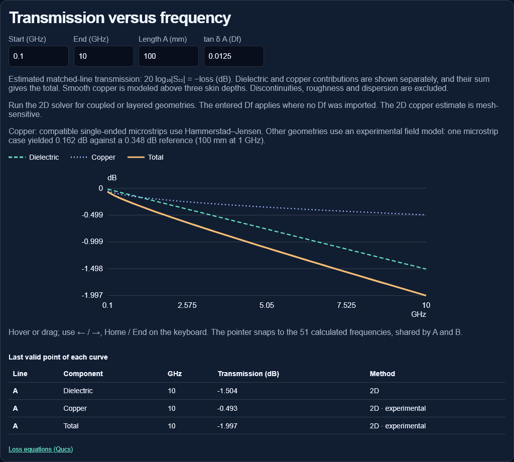
Enter line length in mm, the frequency band in GHz and Df. Three negative-dB curves show dielectric, copper and total contributions. Run the 2D solver first for coupled or layered lines. The entered Df applies where no layer Df was imported.
Compatible single-ended microstrips use Hammerstad–Jensen smooth-copper loss. Other geometries use an experimental field-based copper model. Roughness, dispersion, connectors and discontinuities are excluded. Curves may be unavailable outside their model range, including insufficient copper thickness relative to skin depth.
The plotted transmission assumes a matched line. The table shows each curve’s last valid point. A and B use shared axes for comparison.
Hover or drag to show a vertical pointer and dielectric, copper and total transmission at the same frequency. The pointer snaps to 51 calculated samples and synchronizes A and B. Arrow keys change frequency; Home / End select the bounds. Unavailable contributions show a dash.
Choose Simple or Advanced mode
Simple is the first-visit default: geometry, target, A/B comparison, 2D solving and quick transmission. Advanced reveals fabrication, design studies, technical imports, the stackup library, physical multilayer PCB editor and RLGC / four-port networks.
The browser retains your choice. Returning to Simple hides controls without deleting geometry or materials. A configured broadside pair remains broadside. Active quick-transmission roughness corrections remain enabled and are labeled. Switching away from Advanced cancels calculations in panels that are removed.
Build a multilayer PCB and assign its lines
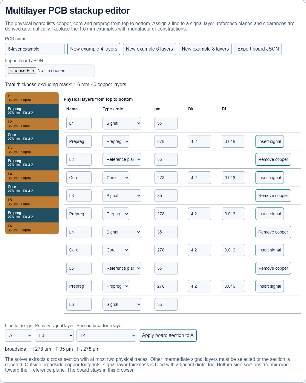
In Advanced mode, the PCB editor offers 4-, 6- and 8-copper-layer examples at 1.6 mm excluding mask. Replace example values with the manufacturer construction. Layers run top to bottom: signal/plane copper, core and prepreg with thickness in µm, Dk and Df. Insert a signal in a dielectric or remove internal copper, up to 16 copper layers.
Choose A or B and a signal layer. Apply derives the cross-section, H, T, dielectric regions and nearest reference planes. Bottom external sections are mirrored toward their reference. For broadside select two signal layers between two planes; model trace 1 is the lower signal and trace 2 the upper. Set lateral offset in geometry.
The solver models at most two traces. An unselected intermediate signal layer prevents extraction. Each dielectric region allows at most six layers. Adjacent dielectric fills the broadside signal-layer thickness outside its copper footprint. Later board changes require Apply again. JSON and local storage retain the board and assignments.
Calculate RLGC, roughness, dispersion and four ports
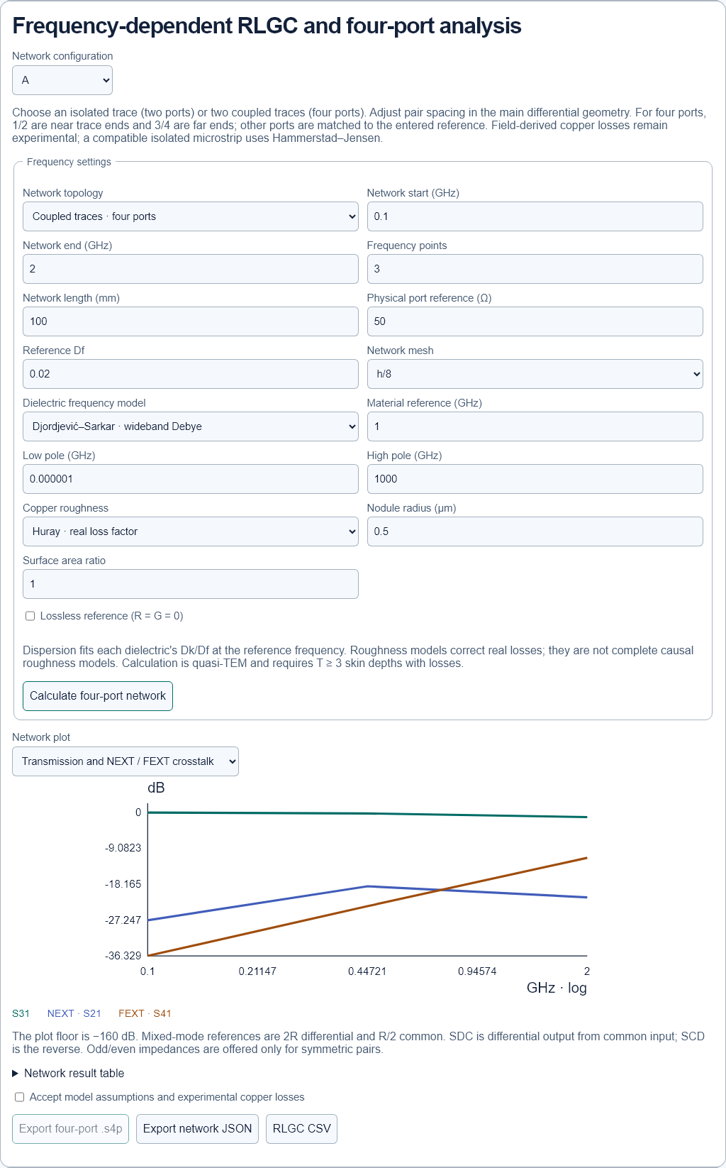
Under RLGC / four ports, select a configuration and a logarithmic band of 3–31 frequencies. Choose an isolated trace with two ports or coupled traces with four ports. The initial choice follows the configuration mode; broadside requires two traces. Set spacing in geometry and enable independent dimensions for unequal traces. Physical ports 1/2 are near trace ends, 3/4 far ends.
Djordjević–Sarkar fits each material to its reference Dk/Df. Set a reference frequency consistent with the supplier data and choose low/high poles; inadmissible fits are rejected. Layer and mask Df override the fallback. Pole values are modeling assumptions, not extra measurements.
Choose smooth copper, Hammerstad with RMS Rq in µm, or Huray with nodule radius in µm and dimensionless surface ratio. These real loss corrections are not a complete causal roughness model. A compatible isolated microstrip uses Hammerstad–Jensen copper loss; other networks use experimental field-derived resistance.
Plots include R, L, G, C, mixed modes, physical transmission S31, near-end crosstalk NEXT=S21 and far-end crosstalk FEXT=S41, with the other ports matched. SDC21 is differential output for common input; SCD21 is the reverse. Mixed references are 2R differential and R/2 common. Complex odd/even impedances are available only for symmetric pairs; differential impedance is then twice Zodd.
Loss calculations require copper at least three skin depths thick and a cross-section small relative to wavelength. Invalid samples remain gaps; the graph floor is −160 dB. Lossless mode sets R=G=0 for comparison. An isolated trace provides S21, scalar RLGC, complex Z0 and .s2p export. Coupled traces provide matrices and .s4p export. Touchstone export requires a complete band and accepted assumptions. JSON preserves geometry/settings and CSV provides SI RLGC matrices. Measured .s4p import is not yet supported.
Check convergence across five meshes
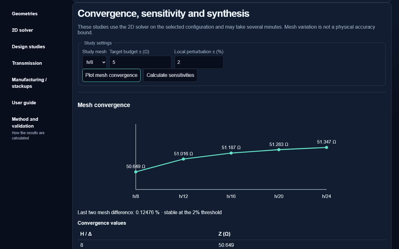
Under Design studies, select A or B and Plot mesh convergence. The cross-section is evaluated at h/8, h/12, h/16, h/20 and h/24. Failed meshes remain missing in both chart and table; line segments never bridge gaps.
The last two meshes share one outer wall. Their difference and a Richardson estimate describe discretization only. A missing final mesh means incomplete refinement. Neither figure bounds material uncertainty or artificial-boundary error.
The solver locally refines both axes near copper, providing at least eight intervals across narrow traces and slots. Global spacing remains h/N. Complex cross-sections can reach the memory cap. Cancel study terminates the worker without applying dimensions.
Quantify sensitivities and manufacturing budgets
Choose a mesh, impedance budget and local perturbation percentage. The target comes from the selected configuration. Calculate sensitivities evaluates relevant parameters at nominal minus and plus the perturbation.
Ranking uses the impedance swing between endpoints. Central derivatives use Ω/µm or Ω/εr. The ±x budget divides remaining target margin by the larger local slope. A nominal value outside the band leaves zero margin. A zero slope or missing solve gives a dash.
This is a one-parameter estimate and can extrapolate beyond the small tested interval. Verify proposed variations in the tolerance study and include multiple parameters. Changing the perturbation can reveal nonlinearity or mesh sensitivity.
Compare width and gap combinations
Select differential mode to enable pair synthesis. Enter W and S bounds and absolute tolerances in µm. Five gaps are explored; bisection finds a target width at each gap.
The stricter CSV and profile minima apply. Bounds include tolerances and trapezoid top width. Candidates must reach target within max(0.25 Ω, 0.2% of target). Four W±ΔW / S±ΔS combinations are then evaluated.
Candidates are ranked by the largest target deviation among nominal and four corners. Incomplete results never pass the band check. Apply changes W and S together. Verify on a fine mesh and include H, T and εr tolerances. Four corners do not guarantee all extrema.
Manage constraints and layer sections
Under Manufacturing / stackups, select a configuration and an example or custom profile. Enter width and gap minima and copper thickness bounds. Examples are not manufacturer capability guarantees. Warnings cover bottom and top width, differential gap, coplanar ground clearance and copper.
Name a stackup and signal layer, for example Acquisition board / L3. Save stores its dielectric/copper construction, mask, materials and constraints. Add more sections for other layers. Applying to A or B preserves routed W, S and G and the current copper inset.
Up to 30 sections stay in this browser. Export library JSON for backup or sharing. Import validates and replaces the current library. When storage is blocked the session remains usable and export retains your work. Each entry describes a cross-section, not an arbitrary multilayer conductor solve.
Import and compare a Touchstone measurement
Under Transmission, open Compare with a Touchstone measurement. Import Touchstone 1.x .s2p using RI, MA or DB, a positive real reference and increasing frequencies. Hz, kHz, MHz and GHz are converted. Limits: 2 MB and 10,000 points. Version 2.x, noise blocks and four-port matrices are unsupported.
Confirm the same line mode, length and measurement reference planes de-embedded to line ends. For differential mode provide an already converted differential two-port; raw .s4p is not processed.
The file reference R recomputes modeled S21 including mismatch. Complex measurement data is interpolated at model frequencies over the shared band only. The chart and table show both transmissions and measured minus modeled dB. Exact zero magnitude gives a dash. Export comparison CSV.
Differences can come from experimental copper losses, materials, roughness, dispersion or measurement effects. They do not quantify solver error alone. Import stays local.
Export a project, report and Touchstone file
Project JSON and CSV export workbench inputs. Reopen project JSON to restore inputs and recompute outputs. The 2D JSON report includes calculation results and tolerance samples. Open the static HTML report in a browser to print or save as PDF.
The design report combines the dimensioned cross-section, provenance, manufacturing rules and completed studies with their settings: convergence, sensitivities and candidate pairs. Open HTML and use Print / Save as PDF. Studies can also be exported as JSON.
Under Transmission, open Touchstone export (.s2p). Select a port reference, typically 50 Ω single-ended or 100 Ω differential. The file contains S11, S21, S12 and S22 with magnitude, phase and mismatch to the chosen reference.
The two ports are the ends of the selected mode. A differential pair exports an equivalent differential two-port. It does not contain a four-conductor matrix or mode conversion. Characteristic impedance is modeled as real and constant over the band.
Every frequency needs both copper and dielectric contributions. To export experimental copper results, enable the corresponding option. The file comments retain that status. Review the model assumptions before using it in a system simulation.
Open the solver · Scientific references · 50 Ω microstrip and differential-pair guides